---
# Contents
* [Introduction](#background)
* [Agent-environment interaction](#agent-env)
* [Reinforcement Learning](#reinforcement)
* [AI\\(\xi\\)](#aixi)
* [Optimality](#optimality)
* [Agents](#agents)
* [Knowledge-seeking agents](#ksa)
* [BayesExp](#bexp)
* [Thompson Sampling](#ts)
* [MDL Agent](#mdl)
# Introduction
[AIXI] and its [variants](#agents) are theoretical models of [artificial general intelligence], formulated under the framework of [reinforcement learning] ([Hutter, 2005]). Informally, these models are attempts to answer the question:
If we make minimal assumptions about our environment, what would constitute rational behavior if computation weren't an issue?
For [fully-observable games] like Chess and Go, optimal play is trivial if you have infinite computing power: just use [minimax](https://en.wikipedia.org/wiki/Minimax) and enumerate the game tree all the way to the end. In contrast, there is no general-purpose algorithm for the case of decision-making under uncertainty and with only partial knowledge. Environments can have traps from which it can be impossible to recover; without knowing _a priori_ which actions lead to traps, an agent will have a tough time learning and performing optimally; this is central to many of the negative results pertaining to this setting, which we will refer to as the general reinforcement learning (GRL) setting.
The purpose of this website is to present AIXI and its relatives in a more accessible way to the AI/RL community, and to demonstrate some of the properties of Bayesian agents in general environments. The [demos] come with short explanations, and some background is laid out (briefly) here.
This page aims to provide an abridged introduction and survey of the GRL literature. For a more comprehensive introduction to these topics, we recommend the PhD theses of [Legg, 2008] and [Leike, 2016], and the author's MSc thesis ([Aslanides, 2016]).
## Agent-environment interaction
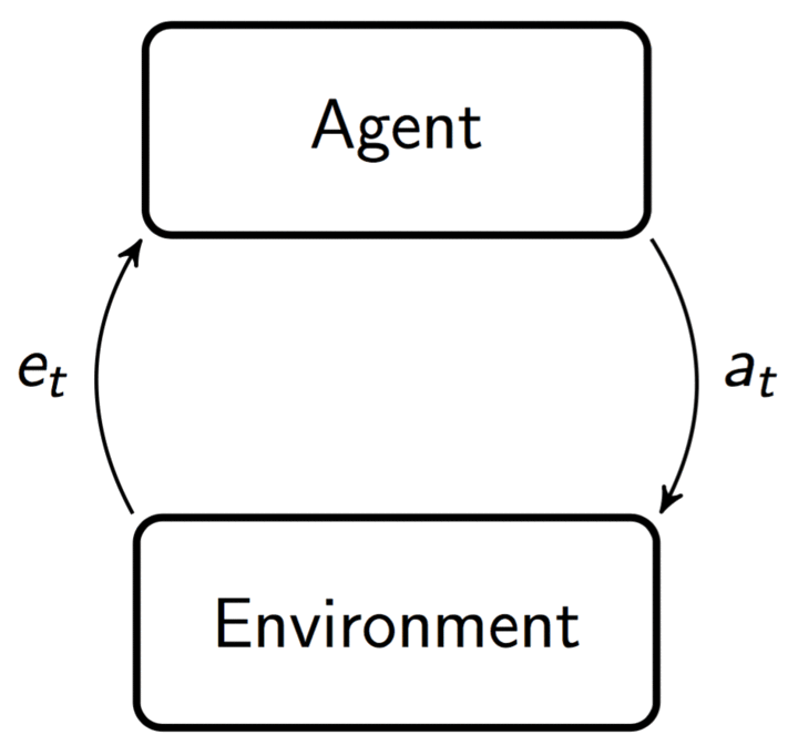
In the standard [reinforcement learning] (RL) framework, the __agent__ and __environment__ play a turn-based game and interact in steps ([Sutton & Barto, 1998]). At time/step/turn \\(t\\), the agent supplies the environment with an __action__ \\(a\_t\\). The environment then performs some computation and returns a __percept__ \\(e_t\\) to the agent, and the step repeats.
The actions live in (usually finite) action space \\(\mathcal{A}\\), and the percepts live in a percept space \\(\mathcal{E}\\). We identify an agent with its __policy__, which in general is a distribution over actions \\(\pi(a\_t\lvert ae\_{<t})\\)
$$
\pi\ :\ \left(\mathcal{A}\times\mathcal{E}\right)^*\mapsto\varDelta\mathcal{A},
$$
where \\(^*\\) is the [Kleene star], and \\(\varDelta \mathcal{X}\\) is the set of probability measures over \\(\mathcal{X}\\). An environment is a distribution over percepts \\(\nu(e\_t\lvert ae\_{<t}a\_t)\\) with
$$
\nu\ :\ \left(\mathcal{A}\times\mathcal{E}\right)^*\times\mathcal{A}\mapsto\varDelta\mathcal{E}.
$$
We call elements of \\(\left(\mathcal{A}\times\mathcal{E}\right)^{\star}\\) (i.e. any finite sequence of action-percept pairs) __histories__. Above we have used
$$
ae\_{<t} \stackrel{.}{=} a\_1e\_1\dots a\_{t-1}e\_{t-1}
$$
to denote a history up to some finite time step \\(t\\).
The agent's policy \\(\pi\\) and the environment's conditional percept distribution \\(\nu\\) induce a measure over histories, which we denote by \\(\nu^\pi\\):
$$
\nu^\pi\left(ae\_{<t}\right) \stackrel{.}{=}\prod\_{k=1}^{t}\pi\left(a\_k\lvert ae\_{<t}\right)\nu\left(e\_k\lvert ae\_{<k}a\_k\right),
$$
which is conveniently expressed as a telescoping product by the [chain rule]. In the general setting, the environment is a [partially observable Markov decision process][POMDP] (POMDP). That is, there is some underlying (hidden) state space \\(\mathcal{S}\\), with respect to which the environment's dynamics are Markovian. The agent cannot observe this state directly, but instead receives (incomplete and noisy) percepts through its sensors. Therefore, the agent must learn and make decisions under uncertainty in order to perform well.
Notes:
* We're slightly abusing notation here: environments are _not_ joint distributions over actions and percepts, and so you should read \\(\nu(e\_t\lvert ae\_{<t}a\_t)\\) as shorthand for \\(\nu(e\_t\lvert e\_{<t} \lvert\lvert a_{1:t})\\); that is, a distribution over percepts conditioned on a sequence of past percepts, and in the context of a sequence of past actions given as _inputs_. The same holds for policies, except with actions and percepts reversed.
* We restrict ourselves to countable percept and action spaces. Although many (but not all) of the important results generalize to continuous spaces, we make this assumption for simplicity.
* For simplicity, we also assume that the action and percept spaces \\(\mathcal{A}\\) and \\(\mathcal{E}\\) are stationary; i.e. they are time-independent and fixed by the environment.
## Reinforcement Learning
Percepts consist of (__observation__, __reward__) pairs \\(e\_k = \left(o\_k,r\_k\right)\\), with integer-valued rewards such that
$$
\mathcal{E} = \mathcal{O}\times\mathbb{Z}.
$$
We make no further assumptions about the observation space \\(\mathcal{O}\\). A good example is the space of \\(M\times N\\)-pixel 8-bit RGB images used in the [Arcade Learning Environment][ALE] (ALE):
$$
\mathcal{O}_{\text{ALE}}=\mathcal{B}^{8\times M\times N\times 3},
$$
where \\(\mathcal{B}\stackrel{.}{=}\lbrace{0,1\rbrace}\\) is the binary alphabet. Now, introduce the __return__, which is the discounted sum of all future rewards:
$$
R\_t \stackrel{.}{=} \sum\_{k=t}^{\infty}\gamma\_k r\_k,
$$
where \\(\gamma\ :\ \mathbb{N}\mapsto[0,1]\\) is a discount function with convergent sum. Now, if our agent is rational in the [Von Neumann-Morgenstern][VNM] sense, it should maximize the expected return, which we call the __value__. The value achieved by policy \\(\pi\\) in environment \\(\nu\\) given history \\(ae\_{<t}\\) is defined as
$$
V^{\pi}\_{\nu}\left(ae\_{<t}\right)\stackrel{.}{=}\mathbb{E}^{\pi}\_{\nu}\left[\left.\sum\_{k=t}^{\infty}\gamma\_{k}r\_{k}\right|ae\_{<t}\right],
$$
where the expectation \\(\mathbb{E}^{\pi}\_{\nu}\\) is with respect to the measure \\(\nu^{\pi}\\). This is often more conveniently expressed recursively:
$$
V^{\pi}\_{\nu}\left(ae\_{<t}\right) = \sum\_{a\_t\in\mathcal{A}}\pi(a\_t\lvert ae\_{<t})\sum\_{e\_t\in\mathcal{E}}\nu(e\_t\lvert ae\_{<t}a\_t)\Big[\gamma\_tr\_t+\gamma\_{t+1}V\_{\nu}^{\pi}(ae\_{1:t})\Big],
$$
which is often referred to as the [Bellman equation]. Now, let \\(\mu\\) be the true environment. The __optimal value__ is the highest value achieved by any policy in this environment; under some pretty reasonable assumptions, this value always exists:
$$
V\_{\mu}^{*}\stackrel{.}{=}\max\_{\pi}V\_{\mu}^{\pi}.
$$
Using the [distributive property] of \\(\max\\) and \\(\sum\\), we can unroll this into the __expectimax__ expression
$$
V\_{\mu}^{*}=\lim\_{m\to\infty}\max\_{a\_{t}\in\mathcal{A}}\sum\_{e\_{t}\in\mathcal{E}}\cdots\max\_{a\_{m}\in\mathcal{A}}\sum\_{e\_{m}\in\mathcal{E}}\sum\_{k=t}^{m}\gamma\_{k}r\_{k}\prod\_{j=t}^{k}\mu\left(e\_{j}\lvert ae\_{<j}a\_{j}\right).
$$
This can be viewed as just a generalization of [minimax] to stochastic environments. In practice, when planning we approximate this computation with [Monte Carlo tree search] (MCTS).
We can now introduce our first theoretical [artificial general intelligent] (AGI) agent: the __informed agent AI__\\(\boldsymbol{\mu}\\). AI\\(\mu\\) is simply the (infeasible) \\(\boldsymbol{\mu}\\)__-optimal policy__:
$$
\pi^{\text{AI}\mu}\stackrel{.}{=}\arg\max\_{\pi}V\_{\mu}^{\pi}.
$$
Of course, we won't know \\(\mu\\) _a priori_ in the general RL setting. Generically, there are two main approaches to learning in the context of RL: __model-based__ and __model-free__. They each make their own sets of assumptions:
* Model-free (e.g. [Q-Learning], [Deep Q-networks]) generally assume the environment is a finite-state MDP
* Model-based (e.g. __Bayesian learning__) assumes the __realizable case__.
The agents we'll be dealing with are all Bayesian.
## Bayesian reinforcement learning
Assume the realizable case: the true environment \\(\mu\\) is contained in some countable __model class__ \\(\mathcal{M}\\). Now, construct a __Bayesian mixture__ over \\(\mathcal{M}\\): a [convex linear combination] of environments:
$$
\xi\left(e\_t\lvert ae\_{<t}a\_t\right)\stackrel{.}{=}\sum\_{\nu\in\mathcal{M}}w\_\nu \nu\left(e\_t\lvert ae\_{<t}a\_t\right).
$$
The weights \\(w\_\nu\equiv\Pr\left(\nu\lvert ae\_{<t}\right)\\) specify the agent's __posterior belief distribution__ over \\(\mathcal{M}\\). By [Cromwell's rule], we require further that the __prior__ weights \\(\Pr(\nu\lvert \epsilon)\\) lie in the interval \\((0,1)\ \forall \nu\in\mathcal{M}\\). Being 'Bayesian' simply means __updating__ these beliefs according to the product rule of probability:
$$
\Pr(\nu\lvert e\_t) = \frac{\Pr(e\_t\lvert \nu)\Pr(\nu)}{\Pr(e\_t)},
$$
which corresponds to performing the update at each step:
$$
w\_\nu\leftarrow\frac{\nu(e\_t)w\_\nu}{\xi(e\_t)}.
$$
## AI\\(\xi\\)
AI\\(\xi\\) is the __Bayes-optimal__ agent. That is, it is the policy that maximizes the \\(\xi\\)-expected return; it is a deterministic policy, given by
$$
\begin{align}
\pi^{\text{AI}\xi} & = \arg\max\_\pi V^\pi\_\xi \\\\
& = \arg\lim\_{m\to\infty}\max\_{a\_{t}\in\mathcal{A}}\sum\_{e\_{t}\in\mathcal{E}}\cdots\max\_{a\_{m}\in\mathcal{A}}\sum\_{e\_{m}\in\mathcal{E}}\sum\_{k=t}^{m}\gamma\_{k}r\_{k}\prod\_{j=t}^{k}\sum\_{\nu\in\mathcal{M}}w\_\nu\nu\left(e\_{j}\lvert ae\_{<j}a\_{j}\right).
\end{align}
$$
It is a universal, parameter-free Bayesian agent, whose behavior is completely specified by its model class \\(\mathcal{M}\\) and choice of prior \\(\lbrace w\_\nu\rbrace\_{\nu\in\mathcal{M}}\\). AI\\(\xi\\)'s big brother is [AIXI] ([Hutter, 2005]), which uses [Solomonoff's universal prior], which mixes over the model class of all computable probability measures:
$$
w\_{\nu} = 2^{-K(\nu)},
$$
where \\(K(\nu)\\) is the [Kolmogorov complexity] of \\(\nu\\). AIXI is hence the 'active' generalization of Solomonoff induction, which is the optimal (but incomputable) inductive learner. AIXI is more commonly written using the formulation of environments as _programs_:
$$
a^{\text{AIXI}}\_{t} = \arg\lim\_{m\to\infty}\max\_{a\_{t}\in\mathcal{A}}\sum\_{e\_{t}\in\mathcal{E}}\cdots\max\_{a\_{m}\in\mathcal{A}}\sum\_{e\_{m}\in\mathcal{E}}\sum\_{k=t}^{m}\gamma\_{k}r\_{k}\sum\_{q\ :\ U(q;a\_{<k})=e\_{<k}\*}2^{-l(q)},
$$
where \\(U\\) is a Universal Turing Machine, and \\(x\*\\) is an infinite string beginning with \\(x\\).
A computable approximation to AIXI is MC-AIXI-CTW ([Veness et al., 2011]), which uses the [Context Tree Weighting] (CTW) algorithm to approximate the induction component of AIXI, and a variant of the UCT MCTS algorithm for planning ([Kocsis & Szepasvari, 2006]).
AIXI is known to have the property of _on-policy value convergence_; that is:
$$
V^{\pi}\_{\xi} - V^{\pi}\_{\mu} \to 0 \quad\text{as }t\to\infty.
$$
This means that AIXI learns how good its policy is, asymptotically. Unfortunately, this is not the same as _asymptotic optimality_, a property that AIXI indeed lacks:
$$
V^{\star}\_{\mu} - V^{\pi}\_{\mu} \to 0 \quad\text{as }t\to\infty.
$$
## Exploration vs exploitation; optimality
One of the central issues in reinforcement learning is the __exploration-exploitation dilemma__: how do you know that what you're doing is the best use of your time? When, and how often, should you take a break from exploiting the best policy you currently know, to go and explore, in the hope of learning more about the environment and discovering a better policy? Also, when you _do_ decide to explore, what strategy should you use to learn the most, given your incomplete knowledge of the environment? These are some of the (many, and big) open problems in the theory of reinforcement learning.
It is now known that [Pareto optimality] is trivial in general environments, and that AIXI can be made to perform arbitrarily badly with a dogmatic prior ([Leike & Hutter, 2015]).
# GRL Agent Zoo
Now, let's introduce AIXI's cousins: knowledge-seeking agents, Thompson sampling, MDL, BayesExp, and Optimistic AIXI. They are all attempts to address the issues with the 'vanilla' Bayesian agent.
## Knowledge-seeking agents
The exploration approach one takes is often critical to one's success in an unknown environment. A principled exploration method for Bayesian agents is by knowledge- or information-seeking. Here, we present the knowledge-seeking agents (KSA) first introduced in [Orseau, 2011] and [Orseau et al., 2013].
First, we generalize our Bayesian reinforcement learner to a Bayesian __utility agent__ that has, in addition to a belief distribution \\(\xi\\), a utility function
$$
u(e\_t\lvert ae\_{<t}a\_t)
$$
which takes the place of the agent's reward signal. A standard reinforcement learner can be expressed as a utility agent by simply setting \\(u(e\_t)=r\_t\\), i.e. to pluck out the reward component of the percept signal. In this setting, the agent is an __expected utility maximizer__, with \\(u(e\_t)\\) replacing \\(r\_t\\) in its value function. Using this formalism, we can construct agents that (in principle, and absent any [self-delusions](https://arxiv.org/pdf/1605.03143.pdf)) care about objective states of the world, and not about some arbitrary reward signal.
Generically, knowledge-seeking agents (KSA; [Orseau, 2011]; [Orseau et al., 2013]) get their utility from gaining information. In the context of Bayesian agents, we express their utility functions in terms of information-theoretic changes to their model. There are three KSA of note:
* Square KSA:
$$
u(e\_t\lvert ae\_{< t} a\_t) = -\xi(e\_t\lvert ae\_{<t}),
$$
* Shannon KSA:
$$
u(e\_t\lvert ae\_{< t} a\_t) = \log\xi(e\_t\lvert ae\_{<t}),
$$
* and Kullback-Leibler KSA:
$$
u(e\_t\lvert ae\_{< t} a\_t) = \text{Ent}(w\lvert ae\_{1:t}) - \text{Ent}(w\lvert ae\_{<, t} a\_t).
$$
These utility functions are so-named because, when we take their \\(\xi\\)-expected value, we get the square- and Shannon-entropies of \\(\xi\\), and the \\(\xi\\)-expected Kullback-Leibler divergence (Lattimore, 2013). Note that these agents differ from AIXI only in their utility functions; they are Bayesian learners, and plan by computing the expectimax expression introduced previously, but substituting \\(u(\cdot\lvert \cdot)\\) for \\(r\\). The value function for a utility agent with utility function \\(u\\) is
$$
V\_{\xi,u}^{\*} = \arg\lim\_{m\to\infty}\max\_{a\_{t}\in\mathcal{A}}\sum\_{e\_{t}\in\mathcal{E}}\cdots\max\_{a\_{m}\in\mathcal{A}}\sum\_{e\_{m}\in\mathcal{E}}\sum\_{k=t}^{m}\gamma\_{k}u(e\_t\lvert ae\_{<k})\prod\_{j=t}^{k}\xi\left(e\_{j}\lvert ae\_{<j}a\_{j}\right).
$$
For the particular case of the KL-KSA, we write its value function as \\(V\_{\xi,\text{IG}}^{\*}\\).
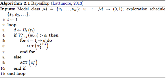
## BayesExp
It turns out that the Bayes agent, AI\\(\xi\\) is not asymptotically optimal in general essentially because one can construct environments in which it fails to explore enough ([Orseau, 2010]). A natural way to extend AI\\(\xi\\) so as to remedy this is to add in bursts of exploration (for an effective horizon -- defined below), when the \\(\xi\\)-expected information gain exceeds some threshold. Thus, we mix the exploratory advantages of knowledge-seeking, at the cost of introducing another parameter (the exploration threshold).
## Thompson Sampling
First, define the \\(\varepsilon\\)-effective horizon:
$$
H\_{t}^{\gamma}(\varepsilon) \stackrel{.}{=} \min\left\lbrace m\ :\ \sum\_{k=m}^{\infty}\gamma\_{t+k}\leq\varepsilon\right\rbrace,
$$
which is the minimum number of steps ahead one needs to plan in order to account for a value of \\((1-\varepsilon)V\_{\nu}^{\pi}\\), for some \\(\varepsilon>0\\). [Thompson Sampling] has been used as an exploration scheme in bandits, and more recently in MDPs. When generalized to POMDPs ([Leike et al., 2016]), Thompson sampling has a simple algorithm: every \\(H\_{t}^{\gamma}\\) steps, sample an environment \\(\rho\\) from the posterior belief distribution \\(w\_{\nu}\\), and use the \\(\rho\\)-optimal policy, re-sample, and repeat.

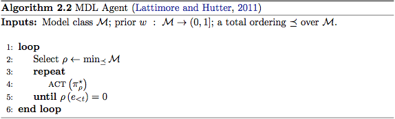
## Minimum Description Length (MDL) Agent
Where AIXI uses a mixture model -- in which it models the world as a weighted average of hypotheses and acts accordingly -- the MDL agent greedily chooses to model the world using the simplest plausible model it knows of. More formally, it chooses the \\(\rho\\)-optimal policy, where \\(\rho\\) is the simplest so-far unfalsified environment.
$$
\rho = \arg\min\_{\nu\in\mathcal{M}\ :\ w\_\nu > 0} K(\nu).
$$
Notice the requirement that \\(w\_\nu > 0\\). This is a clue that the MDL agent will fail in stochastic environments, since its criterion for 'falsification' is too strict: it requires that its posterior assign exactly zero mass to some hypothesis before it's happy to move on and consider an alternative hypothesis.
Of course, in practice (that is, for the purposes of our demos), we can't compute the Kolmogorov complexity of our environment models, so we come up with some other ordering \\(\preceq\\) over \\(\mathcal{M}\\) to approximate it.
---
[reinforcement learning]: https://en.wikipedia.org/wiki/Reinforcement_learning
[artificial general intelligence]: https://en.wikipedia.org/wiki/Artificial_general_intelligence
[Kolmogorov complexity]: https://en.wikipedia.org/wiki/Kolmogorov_complexity
[Q-Learning]: https://en.wikipedia.org/wiki/Q-learning
[Deep Q-networks]: https://www.cs.toronto.edu/~vmnih/docs/dqn.pdf
[AIXI]: https://en.wikipedia.org/wiki/AIXI
[Solomonoff's universal prior]: http://www.scholarpedia.org/article/Algorithmic_probability
[VNM]: https://en.wikipedia.org/wiki/Von_Neumann%E2%80%93Morgenstern_utility_theorem
[minimax]: https://en.wikipedia.org/wiki/Minimax
[Kleene star]: https://en.wikipedia.org/wiki/Kleene_star
[convex linear combination]: https://en.wikipedia.org/wiki/Convex_combination
[Cromwell's rule]: https://en.wikipedia.org/wiki/Cromwell%27s_rule
[Bellman equation]: https://en.wikipedia.org/wiki/Bellman_equation
[Monte Carlo tree search]: https://en.wikipedia.org/wiki/Monte_Carlo_tree_search
[distributive property]: https://en.wikipedia.org/wiki/Distributive_property
[POMDP]: https://en.wikipedia.org/wiki/Partially_observable_Markov_decision_process
[chain rule]: https://en.wikipedia.org/wiki/Chain_rule_(probability)
[ALE]: http://www.arcadelearningenvironment.org/
[artificial general intelligent]: https://en.wikipedia.org/wiki/Artificial_general_intelligence
[Context Tree Weighting]: https://cs.anu.edu.au/courses/comp4620/2015/slides-ctw.pdf
[Pareto optimality]: https://en.wikipedia.org/wiki/Pareto_efficiency
[Andrej Karpathy]: http://cs.stanford.edu/people/karpathy/
[REINFORCEjs]: http://cs.stanford.edu/people/karpathy/reinforcejs/
[Thompson Sampling]: https://en.wikipedia.org/wiki/Thompson_sampling
[fully-observable games]: https://en.wikipedia.org/wiki/Perfect_information
[demos]: demo.html
[Legg, 2008]: http://www.vetta.org/documents/Machine_Super_Intelligence.pdf
[Leike, 2016]: https://jan.leike.name/publications/Nonparametric%20General%20Reinforcement%20Learning%20-%20Leike%202016.pdf
[Aslanides, 2016]: http://aslanides.io/docs/masters_thesis.pdf
[Kocsis & Szepasvari, 2006]: http://ggp.stanford.edu/readings/uct.pdf
[Hutter, 2005]: http://www.hutter1.net/ai/uaibook.htm
[Leike & Hutter, 2015]: http://jmlr.org/proceedings/papers/v40/Leike15.pdf
[Leike et al., 2016]: https://arxiv.org/abs/1602.07905
[Veness et al., 2011]: https://www.jair.org/media/3125/live-3125-5397-jair.pdf
[Orseau, 2011]: http://www.agroparistech.fr/mmip/maths/laurent_orseau/papers/orseau-ALT-2011-knowledge-seeking.pdf
[Orseau et al., 2013]: http://www.hutter1.net/publ/ksaprob.pdf
[Orseau, 2010]: http://link.springer.com/chapter/10.1007/978-3-642-16108-7_28
[Sutton & Barto, 1998]: https://webdocs.cs.ualberta.ca/~sutton/book/the-book.html
[Sunehag & Hutter, 2015]: http://jmlr.org/papers/volume16/sunehag15a/sunehag15a.pdf